Backpropagation is a popular algorithm used in training neural networks, which allows the network to learn from the input data and improve its performance over time. It is essentially a way to update the weights and biases of the network by propagating errors backwards from the output layer to the input layer.
Neural networks can be thought of as very complicated mathematical functions that take in inputs, perform a series of computations, and output predictions or classifications. They can be extremely complex and difficult to understand, especially for larger networks with many layers and thousands or millions of parameters. However, at a high level, they can be thought of as complicated mathematical functions that learn to map inputs to outputs through a process of trial and error.
For simplicity, let’s imagine a very simple function:
\[f(x)=2x^2-3x+4\]This function can be defined in python like this
def f(x):
    return 2*x**2 - 3*x + 4
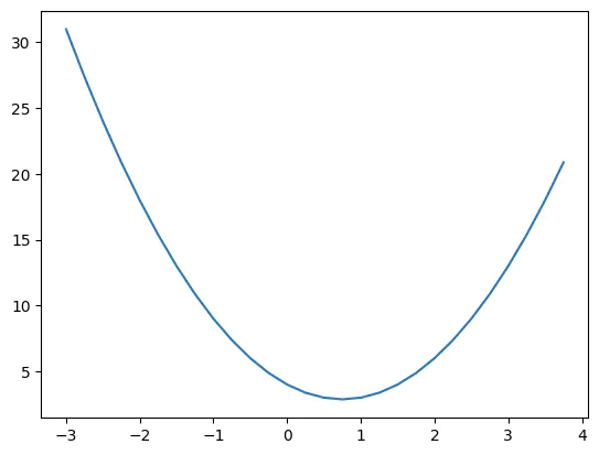
Plot it:
import numpy as np
import matplotlib.pyplot as plt
xs = np.arange(-3, 4, 0.2)
ys = f(xs)
plt.plot(xs, ys)

Let’s now talk about derivatives. What does the derivative of a function tell you? If you head over to the Wikipedia page of Derivatives it says that the derivative of a function measures the sensitivity to change of the function value (output value) with respect to a change in its argument (input value). This means the derivative describes what happens if you add a very small number \(h\) to \(x\), how the function responds and by how much. Does the function go up or down, and how sensitive is it to such changes? This is equivalent to the slope of the tangent line at a given point \(x\).
This means if we know the derivatives, we know how to change the inputs (better: the weights and biases) in a neural network to match a desired output. This is how a neural network is trained.
For simplicity, we illustrate this with the very basic function from above. Please note that in this case we don’t have weights and biases, just inputs. In a regular neural network we usually don’t change the inputs, just the weights in biases.
We can easily calculate \(y\) a any given point \(x\):
f(2)
# 6
f(6)
# 58
f(-2)
# 18
Now let’s define a small number \(h\) and observe how the ouput changes:
h = 0.000001
f(2 + h)
# 6.000005000002001
f(6 + h)
# 58.000021000002
f(-2 + h)
# 17.999989000002003
We observe, that the first two values, 2 and 6, the output increases, while for the last one with \(x=2\), it decreases. According to the Wikipedia definition, the derivative (or the slope) of \(f\) is the limit of
\[\lim_{h\rightarrow 0} \frac{f(x+h)-f(x)}{h}\]In other words, the slope of \(f\) at point \(x\) is the difference between \(f\) at point \(x\) increased by small amount \(h\), and \(f\) at point \(x\), normalized (divided by) \(h\). We can, of course, only approximate this numerically:
h = 0.000001
(f(2 + h) - f(2)) / h
# 5.000002000876691
(f(6 + h) - f(6)) / h
# 21.000002000448603
(f(-2 + h) - f(-2)) / h
# -10.999997996918864
If we make \(h\) smaller and smaller this eventually converges to the true value. From these results, we see that for \(x=-2\) we get a negative slope, while for \(x=2\) and \(x=6\) the slope is positive. At some point, the slope is exactly zero (in our case, at \(x=0.75\)):
h = 0.000000001
(f(0.75 + h) - f(0.75)) / h
# 0.0
Let us now expand this to a more complicated example. We assume three input values \(a\), \(b\), and \(c\), and one output, \(d\), defined as \(d=a\cdot b+c\):
h = 0.0001

#inputs
a = 3.0
b = -2.0
c = 8.0

#output
d = a * b + c
# 2.0
So far we only calculated the derivative of \(f\) with respect to one value, \(x\). Now, we want to calculate the derivatives of \(d\) with respect to all inputs \(a\), \(b\), and \(c\).
# derivative (slope) of d with respect to a
(((a+h) * b + c) - (a * b + c)) / h
# -2.0000000000131024

# derivative (slope) of d with respect to b
((a * (b+h) + c) - (a * b + c)) / h
# 3.00000000000189

# derivative (slope) of d with respect to c
((a * b + (c+h)) - (a * b + c)) / h
# 0.9999999999976694
Let’s look at the individual terms in the first example in more detail:
(a * b + c)
# 2.0

((a+h) * b + c)
# 1.9997999999999996
We observe that if we add a small number \(h\) to \(a\), the output decreases (here, from 2.0 to 1.999). This tells us that the slope will be negative. The exact slope is -2.0 as seen above.
Similarly, for the second value, \(b\), we get
(a * b + c)
# 2.0

(a * (b+h) + c)
# 2.0003
So this output increases from 2.0 to 2.0003 if we add a small number \(h\) to \(b\) meaning a positive slope (here, the exact slope is 3.0).
Let’s work with an even more difficult example now. We define a function with more inputs as follows:
# inputs
a = 3.0
b = -2.0
c = 8.0
d = a * b
e = d + c
f = -2.0
# output
L = e * f
# same as L = (d + c) * f
#           = (a * b + c) * f
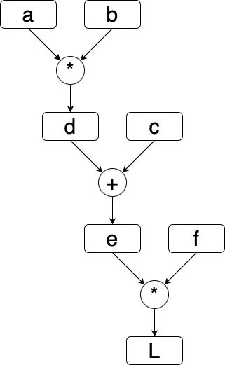
A graph of this function looks like this:

Let’s now calculate the derivatives. Calculating the derivative of \(L\) with respect to \(L\) is easy:
((L + h) - L) / h
# 1.0000000000021103
So the derivative of \(L\) with respect to \(L\) is 1. This is obvious, every derivative with respect to itself is 1, as we can see analytically:
\[\frac{L+h-L}{h} = \frac{h}{h}=1.\]Ok, but what about going back one step in the graph? Let us calculate the derivative of \(L\) with respect to \(e\) and \(f\):
# derivative of L with respect to e
# because L = e * f
(((e+h) * f) - (e * f)) / h
# -2.0000000000042206

# derivative of L with respect to f
(e * (f+h) - e * f) / h
# 1.9999999999997797
As before, we see that \(e\cdot f=-4.0\) and \(((e+h)\cdot f)\) = -4.0002, the slope must negative (because adding \(h\) makes the output more negative). Accordingly, the slope of \(L\) with respect to \(f\) must be positive. In this multiplication example, we saw that the derivative of \(f\) with respect to \(e\) is \(f\) (=-2.0) and the derivative of \(L\) with respect to \(f\) is \(e\) (=2.0). This can be derived analytically as well:
\[\frac{f(x+h)-f(x)}{h}=\frac{(e+h)\cdot f-(e\cdot f)}{h}=\frac{e\cdot f+h\cdot f-e\cdot f}{h}=\frac{h \cdot f}{h}=f\]Let’s go another step backwards in the graph and calculate the derivative of \(L\) with respect to \(d\). We can do this using our well-known formula:
(((d+h) + c) * f - (d + c) * f ) / h
# -1.9999999999
While it’s possible to do it that way for every node in our graph, there’s a more elegant solution. This is the Chain Rule. The chain rule is a fundamental rule in calculus that allows us to calculate the derivative of a composite function. Let’s say we have two functions, \(f(x)\) and \(g(x)\), where \(g(x)\) is the inner function and \(f(x)\) is the outer function. The composite function is then given by \(f(g(x))\). In other words, the derivative of the composite function \(f(g(x))\) is equal to the derivative of the outer function evaluated at the inner function, multiplied by the derivative of the inner function. The chain rule is a powerful tool that allows us to find derivatives of complex functions by breaking them down into simpler parts. In our case, this means for the derivative of \(L\) with respect to \(d\):
\[\frac{dL}{dd}=\frac{dL}{de} \cdot \frac{de}{dd}\]We have already calculated \(\frac{dL}{de}\), and \(\frac{de}{dd}=1\), therefore \(\frac{dL}{dd}=-2\cdot 1=-2\).
Using the chain rule we can caculate the derivatives (or gradients) of all nodes in our graph, backwards starting from L. For example, to calculate \(\frac{dL}{da}\), we need to calculate \(\frac{dL}{da}=\frac{dL}{de} \cdot \frac{de}{dd} \cdot \frac{dd}{da} = -2 \cdot 1 \cdot -2 = 4\). We started with the output \(L\) and moved backwards to calculate the derivative of \(L\) with respect to \(a\).
Hence the term backpropagation.
Here’s how you can do all of the above in few lines using pytorch:
import torch
a = torch.Tensor([3.0])
a.requires_grad = True
b = torch.Tensor([-2.0])
b.requires_grad = True
c = torch.Tensor([8.0])
c.requires_grad = True
d = a * b
e = d + c
f = torch.Tensor([-2.0])
f.requires_grad = True
# output
L = e * f
# calculate the derivatives backwards from L
L.backward()
# show the derivative of dL/da
a.grad.item()
# 4.0
