
In every statistical analysis, the selection of covariates in regression models is akin to navigating a labyrinth. One common heuristic advises controlling for as many variables as possible, under the presumption that it yields more conservative tests of hypotheses. However, this approach is not without pitfalls. Adding wrong or extraneous variables can distort results, introducing spurious effects and even reversing the signs of actual causal relationships. In the following, I will provide an example of how this can happen.
Let’s consider this structural graph:
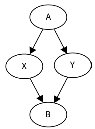
In this example, we want to estimate the effect of \(X\) on \(Y\). However, examining the model structure reveals a clear causal independence between variables \(X\) and \(Y\). There’s no arrow between them, nor is there a directed path that would connect them indirectly. We will now construct four models and investigate the impact of controlling for different variables on the emergence of spurious relationships between \(X\) and \(Y\):
- The first one is a simple model that regresses \(Y\) on \(X\): \(Y \sim X\)
- Then, we’ll add \(A\) to this model: \(Y \sim X + A\)
- Next, we’ll fit a model without \(A\), but \(B\): \(Y \sim X + B\)
- Finally, we’ll build a model with all four variables: \(Y \sim X + A + B\)
Based on your intuition, which of the four models do you believe will accurately represent the causal independence between \(X\) and \(Y\)?
Let’s generate some data:
import numpy as np
import statsmodels.api as sm
np.random.seed(42)

NSAMPLES = 3000

a = np.random.randn(NSAMPLES)
x = 2 * a + np.random.randn(NSAMPLES)
y = 2 * a + np.random.randn(NSAMPLES)
b = 1.7 * x + 0.8 * y
Model 1: \(Y \sim X\)
This is the simple model that regresses \(Y\) on \(X\):
X1 = sm.add_constant(x)
model_1 = sm.OLS(y, X1).fit()
This results in
print(model_1.summary(xname=['const', 'x']))
OLS Regression Results
==============================================================================
Dep. Variable:                      y   R-squared:                       0.630
Model:                            OLS   Adj. R-squared:                  0.630
Method:                 Least Squares   F-statistic:                     5114.
Date:                Mon, 04 Mar 2024   Prob (F-statistic):               0.00
Time:                        12:59:41   Log-Likelihood:                -5173.1
No. Observations:                3000   AIC:                         1.035e+04
Df Residuals:                    2998   BIC:                         1.036e+04
Df Model:                           1
Covariance Type:            nonrobust
==============================================================================
                 coef    std err          t      P>|t|      [0.025      0.975]
------------------------------------------------------------------------------
const          0.0465      0.025      1.874      0.061      -0.002       0.095
x              0.8030      0.011     71.510      0.000       0.781       0.825
==============================================================================
Omnibus:                        3.944   Durbin-Watson:                   2.047
Prob(Omnibus):                  0.139   Jarque-Bera (JB):                4.150
Skew:                           0.043   Prob(JB):                        0.126
Kurtosis:                       3.161   Cond. No.                         2.21
==============================================================================
Apparently, this model finds a spurious effect of \(X\) on \(Y\), indicated by the low p-value (< 0.001).
Model 2: \(Y \sim X + A\)
What about model 2, we add \(A\) as a covariate:
X2 = sm.add_constant(np.stack([x, a]).T)
model_2 = sm.OLS(y, X2).fit()
print(model_2.summary(xname=['const', 'x', 'a']))
OLS Regression Results
==============================================================================
Dep. Variable:                      y   R-squared:                       0.789
Model:                            OLS   Adj. R-squared:                  0.789
Method:                 Least Squares   F-statistic:                     5600.
Date:                Mon, 04 Mar 2024   Prob (F-statistic):               0.00
Time:                        13:11:43   Log-Likelihood:                -4333.0
No. Observations:                3000   AIC:                             8672.
Df Residuals:                    2997   BIC:                             8690.
Df Model:                           2
Covariance Type:            nonrobust
==============================================================================
                 coef    std err          t      P>|t|      [0.025      0.975]
------------------------------------------------------------------------------
const          0.0036      0.019      0.190      0.850      -0.033       0.040
x              0.0192      0.019      1.034      0.301      -0.017       0.056
a              1.9714      0.042     47.435      0.000       1.890       2.053
==============================================================================
Omnibus:                        0.439   Durbin-Watson:                   2.023
Prob(Omnibus):                  0.803   Jarque-Bera (JB):                0.394
Skew:                           0.024   Prob(JB):                        0.821
Kurtosis:                       3.028   Cond. No.                         5.70
==============================================================================
This model seems to recognize the causal independence of \(X\) and \(Y\) correctly (large p-value for \(X\), suggesting the lack of significance).
Model 3: \(Y \sim X + B\)
In this model, we add \(B\) as a covariate instead of \(A\):
X3 = sm.add_constant(np.stack([x, b]).T)
model_3 = sm.OLS(y, X3).fit()
print(model_3.summary(xname=['const', 'x', 'b']))
OLS Regression Results
==============================================================================
Dep. Variable:                      y   R-squared:                       1.000
Model:                            OLS   Adj. R-squared:                  1.000
Method:                 Least Squares   F-statistic:                 1.002e+32
Date:                Mon, 04 Mar 2024   Prob (F-statistic):               0.00
Time:                        13:18:27   Log-Likelihood:                 92892.
No. Observations:                3000   AIC:                        -1.858e+05
Df Residuals:                    2997   BIC:                        -1.858e+05
Df Model:                           2
Covariance Type:            nonrobust
==============================================================================
                 coef    std err          t      P>|t|      [0.025      0.975]
------------------------------------------------------------------------------
const       2.932e-16   1.58e-16      1.858      0.063   -1.63e-17    6.03e-16
x             -2.1250   3.48e-16  -6.11e+15      0.000      -2.125      -2.125
b              1.2500   1.45e-16   8.61e+15      0.000       1.250       1.250
==============================================================================
Omnibus:                        1.629   Durbin-Watson:                   2.010
Prob(Omnibus):                  0.443   Jarque-Bera (JB):                1.563
Skew:                           0.038   Prob(JB):                        0.458
Kurtosis:                       3.082   Cond. No.                         13.6
==============================================================================
Again, this model finds a spurious effect of \(X\) on \(Y\), indicated by the low p-value (< 0.001). Interestingly, compared with model 1, this time the effect is negative.
Model 4: \(Y \sim X + A + B\)
Time for the last model which includes both \(A\) on \(B\).
X4 = sm.add_constant(np.stack([x, a, b]).T)
model_4 = sm.OLS(y, X4).fit()
print(model_4.summary(xname=['const', 'x', 'a', 'b']))
OLS Regression Results
==============================================================================
Dep. Variable:                      y   R-squared:                       1.000
Model:                            OLS   Adj. R-squared:                  1.000
Method:                 Least Squares   F-statistic:                 1.487e+32
Date:                Mon, 04 Mar 2024   Prob (F-statistic):               0.00
Time:                        13:22:49   Log-Likelihood:                 94094.
No. Observations:                3000   AIC:                        -1.882e+05
Df Residuals:                    2996   BIC:                        -1.882e+05
Df Model:                           3
Covariance Type:            nonrobust
==============================================================================
                 coef    std err          t      P>|t|      [0.025      0.975]
------------------------------------------------------------------------------
const       2.515e-16   1.06e-16      2.377      0.018     4.4e-17    4.59e-16
x             -2.1250   2.45e-16  -8.69e+15      0.000      -2.125      -2.125
a           6.661e-16    3.1e-16      2.147      0.032    5.79e-17    1.27e-15
b              1.2500   1.29e-16    9.7e+15      0.000       1.250       1.250
==============================================================================
Omnibus:                        0.182   Durbin-Watson:                   2.031
Prob(Omnibus):                  0.913   Jarque-Bera (JB):                0.171
Skew:                          -0.018   Prob(JB):                        0.918
Kurtosis:                       3.003   Cond. No.                         19.0
==============================================================================
This model finds a spurious effect of \(X\) on \(Y\), again with a negative effect.
Conclusion
The only model that recognized the causal independence of \(X\) and \(Y\) correctly (large p-value for \(X\), suggesting the lack of significance) is the second model \(Y \sim X + A\). Interestingly, all other statistical control schemes yielded invalid results, including the model without any additional variables accounted for.
Why did controlling for \(A\) succeed while other approaches failed? There are three key factors to consider:
- Confounding Control: \(A\) serves as a confounder between \(X\) and \(Y\), and we need to control for it in order to remove confounding.
- Collider Effect: \(X\), \(Y\), and \(B\) exhibit a pattern known as a collider. Remarkably, this pattern facilitates the flow of information between the parent variables (\(X\) and \(Y\)) when the child variable (\(B\)) is controlled for—a stark contrast to the outcome when \(A\) is controlled for.
- Effect of Variable Control: Interestingly, not controlling for any variable produces the same outcome regarding the significance of \(X\) as controlling for both \(A\) and \(B\). While the coefficient results may differ, focusing on the structural properties of the system reveals that the effects of controlling for \(A\) and \(B\) are diametrically opposite, effectively nullifying each other’s impact.
References
Cinelli, C., Forney, A., & Pearl, J. (2022). A Crash Course in Good and Bad Controls. Sociological Methods & Research, 0 (0), 1-34 https://ftp.cs.ucla.edu/pub/stat_ser/r493.pdf