
Regression is a statistical technique that helps you to estimate the relationship between a dependent variable and one or more independent variables. It is basically the simplest machine learning algorithm you can imagine. For example, you can use regression to find out how the price of a house depends on its size, location, number of rooms, etc.
There are different types of regression, such as linear regression, logistic regression, nonlinear regression, etc. Each type has its own assumptions and methods of fitting the data. In this article, I will focus on linear regression, which is the simplest and most common type of regression.
Simple linear regression assumes that there is a linear relationship between the dependent variable and the independent variable, i.e., the data points can be approximated by a straight line. The equation of this line is:
\[y = \beta_o + \beta_1 x + \varepsilon\]where:
- \(y\) is the dependent variable
- \(x\) is the independent variable
- \(\beta_0\) is the intercept term, i.e. the value of \(y\) when \(x\) is zero
- \(\beta_1\) is the slope term, i.e., the change in \(y\) when \(x\) changes by one unit
- \(\varepsilon\) is the error term, i.e. the difference between the actual and predicted values of \(y\)
The goal of simple linear regression is to find the values of \(\beta_0\) and \(\beta_1\) that minimize the sum of squared errors (SSE),
i.e., the sum of the squares of ϵ for all data points.
This can be done using various methods, such as ordinary least squares (OLS), gradient descent, etc.
Here, we will use the two deep learning libraries `
` and tensorflow.
PyTorch has the torch.nn.Linear() module, also known as a feed-forward layer or fully connected layer, for this task.
This layer implements a matrix multiplication between an input \(x\) and a weights matrix \(W\):
Here, \(b\) would be the bias (same as \(\varepsilon\) above), and \(y\) is the outcome. In neural networks, the weight matrix \(W\) is usually initialized randomly and gets adjusted as the networks learns to better represent patterns in the data.
First, recall how matrix multiplication works. This animation illustrates it:
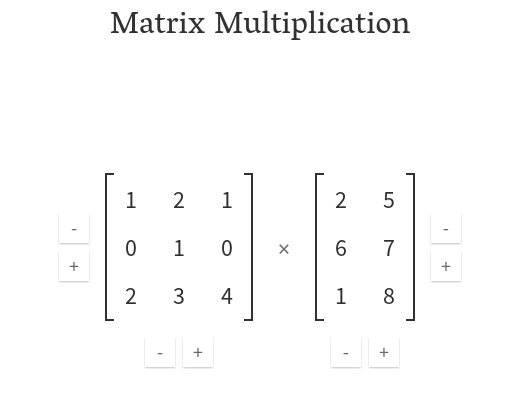
In PyTorch, let’s define two tensors (matrices) A and B:
import torch

A = torch.tensor([[1, 2, 1],
                  [0, 1, 0],
                  [2, 3, 4]])

B = torch.tensor([[2, 5],
                  [6, 7],
                  [1, 8]])
Matrix multiplication (aka the dot product) can be done in PyTorch in several ways:
X @ W
# tensor([[15, 27],
#         [ 6,  7],
#         [26, 63]])

torch.matmul(X, W)
# tensor([[15, 27],
#         [ 6,  7],
#         [26, 63]])

torch.mm(X, W)
# tensor([[15, 27],
#         [ 6,  7],
#         [26, 63]])
Ok, now we know how matrix multiplication works. Using this knowledge, let’s now build a real linear regression model in PyTorch.
First, create some data. We define fixed values for the weight and bias parameters. These are variables our model should learn later on.
weight = 0.8
bias = 0.2

X = torch.arange(start=0, end=2, step=0.02)
y = X * weight + bias
X
# (tensor([0.0000, 0.0200, 0.0400, 0.0600, 0.0800, 0.1000, 0.1200, 0.1400, 0.1600,
#          0.1800, 0.2000, 0.2200, 0.2400, 0.2600, 0.2800, 0.3000, 0.3200, 0.3400,
#                                         ...
#          1.6200, 1.6400, 1.6600, 1.6800, 1.7000, 1.7200, 1.7400, 1.7600, 1.7800,
#          1.8000, 1.8200, 1.8400, 1.8600, 1.8800, 1.9000, 1.9200, 1.9400, 1.9600,
#          1.9800]),
y
# tensor([0.2000, 0.2160, 0.2320, 0.2480, 0.2640, 0.2800, 0.2960, 0.3120, 0.3280,
#         0.3440, 0.3600, 0.3760, 0.3920, 0.4080, 0.4240, 0.4400, 0.4560, 0.4720,
#                                         ...
#          1.4960, 1.5120, 1.5280, 1.5440, 1.5600, 1.5760, 1.5920, 1.6080, 1.6240,
#          1.6400, 1.6560, 1.6720, 1.6880, 1.7040, 1.7200, 1.7360, 1.7520, 1.7680,
#          1.7840]))
Split the data into train and test set
# Split into train and test
train_split = int(0.8 * len(X)) # 80% of data used for training set, 20% for testing
X_train, y_train = X[:train_split], y[:train_split]
X_test, y_test = X[train_split:], y[train_split:]

len(X_train), len(y_train), len(X_test), len(y_test)
# (80, 80, 20, 20)
We have 80 samples in the training set and 20 in the test set. Visualize the data:
import matplotlib.pyplot as plt
plt.figure(figsize=(9, 6))
# plot training data in blue
plt.scatter(X_train, y_train, c='b', label='Training data')
# plot test data in green
plt.scatter(X_test, y_test, c='g', label='Testing data')
# add the legend
plt.legend();

For this exercise, we train the model on the blue data points and try to predict the green points. This should be fairly easy, it’s extending a line, right?
PyTorch
The first step in creating a torch model is define the linear regression model class.
In PyTorch, almost everything is a Module and we inherit from this class.
from torch import nn
# Create a Linear Regression model class
class LinearRegressionModel(nn.Module):
    def __init__(self):
        super().__init__()
        self.weights = nn.Parameter(torch.randn(1, dtype=torch.float),
                                   requires_grad=True)

        self.bias = nn.Parameter(torch.randn(1, dtype=torch.float),
                                requires_grad=True)

    def forward(self, x: torch.Tensor) -> torch.Tensor:
        return self.weights * x + self.bias
In this class, we defined both weights and bias and initilazed them randomly. We set requires_grad=True so the gradients can be updated during training. The forward() function returns the matrix multiplication (dot product) of x and the weights.
Both weights and bias are initilized randomly, so far the model has not learned anything.
Let’s see what our untrained model with random weights predicts on the test data:
with torch.inference_mode():
    y_preds = LinearRegressionModel()(X_test)
y_preds
# tensor([1.5488, 1.5455, 1.5422, 1.5390, 1.5357, 1.5324, 1.5292, 1.5259, 1.5226,
#        1.5194, 1.5161, 1.5129, 1.5096, 1.5063, 1.5031, 1.4998, 1.4965, 1.4933,
#        1.4900, 1.4868])
if we compare this with the true values, it’s pretty far away
y_test
# tensor([1.4800, 1.4960, 1.5120, 1.5280, 1.5440, 1.5600, 1.5760, 1.5920, 1.6080,
#         1.6240, 1.6400, 1.6560, 1.6720, 1.6880, 1.7040, 1.7200, 1.7360, 1.7520,
#         1.7680, 1.7840])
Before we move on, I previously said that PyTorch has a Linear() layer built in, but we haven’t used it so far.
Let’s change this and modify our class to use the standard torch.nn.Linear():
class LinearRegressionModel(nn.Module):
    def __init__(self):
        super().__init__()
        # Use built-in nn.Linear()
        self.linear_layer = nn.Linear(in_features=1,
                                      out_features=1)

    def forward(self, x: torch.Tensor) -> torch.Tensor:
        return self.linear_layer(x)
If we check the model parameters, we see that this module has weights and bias already built in and initializes them randomly:
model = LinearRegressionModel()
model, model.state_dict()
# (LinearRegressionModel(
#    (linear_layer): Linear(in_features=1, out_features=1, bias=True)
#  ),
#  OrderedDict([('linear_layer.weight', tensor([[-0.1230]])),
#               ('linear_layer.bias', tensor([0.7478]))]))
Remember that the true values for weight and bias were 0.8 and 0.2, respectively. The random values are pretty far off, it’s not surprising the predictions are bad.
To train our model, we need to define the loss function and the optimizer. We use the L1Loss which corresponds to the mean absolute error (MAE).
As an optimizer, we use stochastic gradient descent (SGD) with a learning rate of 0.01. This value is usually a good starting point.
# create loss function
loss_fn = nn.L1Loss()

# define optimizer
optimizer = torch.optim.SGD(params=model.parameters(), lr=0.01)
Finally, we need to the define the training loop. In PyTorch, this involves the following steps:
- Forward pass - You pass the input data to the model and get the output. This is done by simply calling the model object with the input as an argument, e.g.
model = model(input). Internally, this executes theforward()function - Calculate the loss - You calculate the loss (or error) between the output and the target (or label) using a loss function, e.g.,
loss = criterion(output, target). PyTorch provides various loss functions in thetorch.nn module. - Zero the gradients - You set the gradients of all the model parameters to zero before the backward pass. This is because PyTorch accumulates gradients by default, so you need to clear them before each iteration. This is done by calling
model.zero_grad()oroptimizer.zero_grad(), where optimizer is an instance of a PyTorch optimizer class that updates the model parameters based on the gradients. - Backpropagate the loss - You compute the gradients of all the model parameters with respect to the loss by calling
loss.backward(). This uses automatic differentiation to efficiently calculate the gradients. - Update the gradients - You update the model parameters using an optimization algorithm, such as stochastic gradient descent (SGD), Adam, etc. PyTorch provides various optimizers in the
torch.optimmodule that implement different optimization algorithms. You need to create an optimizer object and pass it the model parameters and other hyperparameters, such as learning rate, weight decay, etc. Then you calloptimizer.step()to update the parameters based on the gradients.
# define the epochs (how often the models sees the data)
epochs = 500

device = "cpu"
# alternatively
# device = torch.device("cuda" if torch.cuda.is_available() else "cpu")
# Put data on the device
# Reshape the data with unsqueeze, required for the Linear module
X_train = X_train.unsqueeze(dim=1).to(device)
X_test = X_test.unsqueeze(dim=1).to(device)
y_train = y_train.unsqueeze(dim=1).to(device)
y_test = y_test.unsqueeze(dim=1).to(device)

for epoch in range(epochs):
    ### Training
    model.train()

    # 1. Forward pass
    y_pred = model(X_train)

    # 2. Calculate loss
    loss = loss_fn(y_pred, y_train)

    # 3. Zero grad optimizer
    optimizer.zero_grad()

    # 4. Loss backward
    loss.backward()

    # 5. Perform optimization step
    optimizer.step()

    ### Testing
    model.eval() # inference
    # 1. Forward pass
    with torch.inference_mode():
        test_pred = model(X_test)

        # 2. Calculate the loss
        test_loss = loss_fn(test_pred, y_test)

    # print loss every 100 epochs
    if epoch % 100 == 0:
        print(f"Epoch: {epoch} | Train loss: {loss} | Test loss: {test_loss}")

# Epoch: 0 | Train loss: 0.8663485646247864 | Test loss: 2.121262311935425
# Epoch: 100 | Train loss: 0.2715910077095032 | Test loss: 0.6603046655654907
# Epoch: 200 | Train loss: 0.17166011035442352 | Test loss: 0.3427932560443878
# Epoch: 300 | Train loss: 0.08071128278970718 | Test loss: 0.15863864123821259
# Epoch: 400 | Train loss: 0.004712129943072796 | Test loss: 0.01894279755651951
# Epoch: 500 | Train loss: 0.004712129943072796 | Test loss: 0.01894279755651951
We see that the model converged after around 400 epochs as the test loss does not change any more.
Again we can check the learned parameters weight and bias:
model.state_dict()
# OrderedDict([('linear_layer.weight', tensor([[0.8005]])), ('linear_layer.bias', tensor([0.2043]))])
Remember that we generated the data with weights=0.8 and bias=0.2 so this is pretty close!
Finally, let’s make predictions
# activate evaluation mode
model.eval()

# predict on the test data
with torch.inference_mode():
    y_preds = model(X_test)
y_preds
# tensor([[1.4851],
#         [1.5011],
#         [1.5171],
#         [1.5331],
#         [1.5491],
#         [1.5652],
#         [1.5812],
#         [1.5972],
#         [1.6132],
#         [1.6292],
#         [1.6452],
#         [1.6612],
#         [1.6772],
#         [1.6932],
#         [1.7092],
#         [1.7253],
#         [1.7413],
#         [1.7573],
#         [1.7733],
#         [1.7893]])
Visualize the predictions
plt.figure(figsize=(9, 6))
# Plot training data in blue
plt.scatter(X_train, y_train, c='b', label='Training data')
# Plot test data in green
plt.scatter(X_test, y_test, c='g', label='Testing data')
# Plot predictions in red
plt.scatter(X_test, y_preds, c='r', label='Predictions')
# Show the legend
plt.legend();

The predictions are almost spot on!
Tensorflow
For completeness, let’s fit the same model in Tensorflow. Through the keras API, fitting a linear model is super simple:
import tensorflow as tf

model_tf = tf.keras.Sequential([
  tf.keras.layers.Dense(1)
])

# Compile the model
model_tf.compile(loss=tf.keras.losses.mae,
                optimizer=tf.keras.optimizers.SGD(),
                metrics=['mae'])

# Fit the model
model_tf.fit(tf.expand_dims(tf.convert_to_tensor(X_train.numpy()), axis=-1), y_train.numpy(), epochs=300, verbose=1)

# Epoch 298/300
# 3/3 [==============================] - 0s 4ms/step - loss: 0.0080 - mae: 0.0080
# Epoch 299/300
# 3/3 [==============================] - 0s 4ms/step - loss: 0.0088 - mae: 0.0088
# Epoch 300/300
# 3/3 [==============================] - 0s 5ms/step - loss: 0.0077 - mae: 0.0077
Tensorflow has a Dense layer that’s quite similar to the Linear layer in PyTorch.
Note that Tensorflow also requires an extra dimension for the training data (tf.expand_dims).
To convert the data from PyTorch to Tensorflow, I first made them a numpy array.
Let’s predict from this Tensorflow model:
y_preds_tf = model_tf.predict(X_test.numpy())
and plot the results:
plt.figure(figsize=(9, 6))
# Plot training data in blue
plt.scatter(X_train, y_train, c='b', label='Training data')
# Plot test data in green
plt.scatter(X_test, y_test, c='g', label='Testing data')
# Plot predictions in red
plt.scatter(X_test, y_preds_tf, c='r', label='Predictions TF')
# Show the legend
plt.legend();

Also quite good!