
I’ve been playing around with the Stan probabilistic programming language for full Bayesian statistical inference lately. Stan has nice R interface in the rstan package.
This will be (hopefully) the start of a small serious where we fit some simple models using Stan.
We start with a Gamma GLM.
First we generate some data:
set.seed(41)
N <- 500
dat <- data.frame(x1=runif(N,-1,1),x2=runif(N,-1,1))
X <- model.matrix(~x1*x2,dat) # the model matrix
K <- dim(X)[2] #number of regression params
betas <- runif(K,-1,1) #regression parameters
mus <- exp(X%*%betas)
shape <- 10
y <- rgamma(N, rate = shape / mus, shape = shape)
We now have a model matrix $X$, shape = 10, outcome $y$ and a beta vector -0.0702916, 0.584457, -0.0801521, 0.0893137 and try to estimate the true parameters.
Here is the Stan model, defined as a string
stan_code <- "
data {
  int<lower=0> N;
  int<lower=0> K;
  matrix[N,K] X; // predictor matrix
  vector[N] y;
}
parameters {
  vector[K] betas;
  real<lower=0.001,upper=100> shape;
}
model {
  for(k in 1:K)
    betas[k] ~ normal(0,100);
  shape ~ cauchy(0,2.5);
  for(i in 1:N)
    y[i] ~ gamma(shape, (shape / exp(X[i,] * betas)));
}
"
Execute the stan function from rstan using four chains on four cores
library(rstan)
m <- stan(model_code = stan_code, data = list(X=X, K=K, y = y, N = N),
               chains = 4, cores =4)
print(m, digits=4)
## Inference for Stan model: 2debbac23de3eb7ab487a1468524ae7d.
## 4 chains, each with iter=2000; warmup=1000; thin=1;
## post-warmup draws per chain=1000, total post-warmup draws=4000.
##
##              mean se_mean     sd     2.5%      25%      50%      75%
## betas[1]  -0.0891  0.0003 0.0146  -0.1173  -0.0991  -0.0890  -0.0787
## betas[2]   0.5672  0.0004 0.0254   0.5179   0.5498   0.5679   0.5845
## betas[3]  -0.1092  0.0004 0.0253  -0.1586  -0.1267  -0.1093  -0.0922
## betas[4]   0.0687  0.0008 0.0439  -0.0195   0.0394   0.0684   0.0978
## shape      9.7702  0.0113 0.6286   8.5317   9.3401   9.7632  10.1951
## lp__     -90.4331  0.0429 1.6759 -94.6098 -91.2834 -90.1007 -89.2248
##             97.5% n_eff   Rhat
## betas[1]  -0.0617  3149 0.9993
## betas[2]   0.6161  3444 1.0014
## betas[3]  -0.0588  3408 0.9996
## betas[4]   0.1536  2914 1.0002
## shape     11.0178  3084 1.0004
## lp__     -88.2414  1526 1.0009
##
## Samples were drawn using NUTS(diag_e) at Thu Feb 11 13:36:01 2016.
## For each parameter, n_eff is a crude measure of effective sample size,
## and Rhat is the potential scale reduction factor on split chains (at
## convergence, Rhat=1).
If you compare the estimated shape and betas, you see that are almost spot on.
Let’s see a trace plot of the MCMC chains:
traceplot(m)
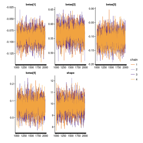
Looks like a nice caterpillar plot, all good.