
Xgboost is short for eXtreme Gradient Boosting and currently one of best machine learning packages available for R. It is fast, memory efficient and can handle huge amounts of data and won several kaggle competitions..
Xgboost is now on CRAN and can be installed from there.
Installation
library(xgboost)
The data
As an example data set we use the Adult data from the arules package:
library(arules)
data("AdultUCI")
We also load the caret package for the createDataPartition() function we use later.
library(caret)
This data set is quite large, with over 48000 observations of 15 variables. Unfortunately it has a huge amount of missings, so we have to delete these oberservations. We delete all rows with missing values:
data <- AdultUCI[complete.cases(AdultUCI),]
We still have 30162 observations left. The variable we want to predict is income which can take two states, small and large, so we are facing a binary classification problem.
A simple prediction model
We split our data in a training and test set. Xgboost uses its own data structure called xgb.DMatrix. R’s matrix structure also works but xgb.DMatrix is preferred.
set.seed(41)
idx <- createDataPartition(data$income, p = 0.85, list = FALSE, time = 1)
labels <- seq_along(levels(data$income))[data$income] - 1  # save the labels
data$income <- NULL                                        # now delete them
train <- model.matrix(~ . + 0, data[idx,])               # the training set
test <- model.matrix(~ . + 0, data[-idx,])               # the test set
dtrain <- xgb.DMatrix(data = train, label = labels[idx])
dtest <- xgb.DMatrix(data = test, label = labels[-idx])
We then set the Xgboost parameters, note that we set auc as the evaluation metric. Xgboost has some built-in evaluation metrics, this is also the reason why we specified the label parameter in dtest. Usually this information is not available for the test set and can be omitted.
For evaluation we will later use the ROCR package, but we keep this for cosmetical reasons.
param <- list(objective="binary:logistic", eta=0.01,
               min_child_weight=4, subsample=0.85, max_delta_step=3,
               colsample_bytree=0.3, max_depth=3, scale_pos_weight=1, eval_metric="auc")
num_rounds <- 5000
More information on these parameters can be found here.
Finally, we can train our model:
mod <- xgb.train(params = param, data = dtrain, nrounds = num_rounds)
We then predict on the test set:
pred <- predict(mod, dtest)
To evaluate the AUROC we use the package ROCR:
library(ROCR)
auc.tmp <- prediction(pred, labels[-idx])
auc <- performance(auc.tmp, "auc")
auc@y.values
## [[1]]
## [1] 0.9302011
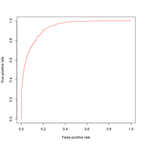
We already get a pretty good AUC value of 0.9302011, here is the plot:
auc <- performance(auc.tmp, "tpr", "fpr")
plot(auc,col=rainbow(10))
A more advanced model
The main problem in boosting is when to stop the boosting iterations. Too many interations can lead to overfitting. xgb.train can follow the progress of the learning process after each round, so if we provide a second data set that is already classified, Xgboost can evaluate the model on this data and find the ideal stopping iterations.
To do this, we split the training data set again, in a new (smaller) training set and a validation set. Before, we had 25638 observations in our training set. We now use the first 2000 observations from this set for early stopping:
valid <- train[1:2000,]
dvalid <- xgb.DMatrix(valid, label = labels[idx[1:2000]])
train2 <- train[-(1:2000),]
dtrain2 <- xgb.DMatrix(train2, label = labels[setdiff(idx, idx[1:2000])])
In addition, we have to specify a watchlist
watchlist <- list("val"=dvalid, "train"=dtrain2)
Then we train the new model. Because of early stopping we can safely increase the number of boosting iterations:
num_rounds <- 8000
mod2 <- xgb.train(param, dtrain2, nthread=2, nrounds = num_rounds, watchlist = watchlist,
                  early.stop.round = 200, maximize = TRUE)
We predict again:
pred2 <- predict(mod2, dtest)
We compute the AUROC again:
auc.tmp <- prediction(pred2, labels[-idx])
auc <- performance(auc.tmp, "auc")
auc@y.values
## [[1]]
## [1] 0.930055
We now get an AUC value of 0.930055. This is not an improvement, it is even slightly worse than our prediction from above. The reason for this may be because
- the AUC is already very high. Remember, a perfect value would be 1.0, this is already close.
- We lose some important information in the training set as we hold out 2000 observations for early stopping
To address the second point, we now build 10 new models with different training/validation splits.
Let’s start from the beginning, otherwise our code will soon become very ugly. idx contains all indices of the test data. We split train in 10 parts (10 folds), so each validation part has 2563 observations. This is easy with the createFolds() function in the caret package:
folds <- createFolds(labels[idx], k = 10)
fmat <- do.call(cbind, folds)
As a result, we get a list of length 10 that holds all the required indices of each fold. I converted the folds to a matrix fmat for easier indexing (because the observations cannot be divided by 10 evenly, some folds contain one repeated observation).
Let’s build our 10 new training and validation sets:
for(i in 1:10) {
  tr <- train[as.vector(fmat[,-i]),]
  v <- train[as.vector(fmat[,i]),]
  eval(parse(text=paste0("dval",i,"<-", "xgb.DMatrix(v, label = labels[idx[as.vector(fmat[,i])]])")))
  eval(parse(text=paste0("dtr",i,"<-", "xgb.DMatrix(tr, label = labels[idx[as.vector(fmat[,-i])]])")))
}
We have to build 10 watchlists, too:
for(k in 1:10) {
  eval(parse(text=paste0("watchlist",k,"<-list('train'=dtr",k,",'val'=dval",k,")")))
}
Then, train all models:
for(n in 1:10) {
  eval(parse(text=paste0("m",n,"<-xgb.train(param, dtr",n,",nthread=2, nrounds = num_rounds, watchlist = watchlist",n,",early.stop.round = 200, maximize = TRUE)")))
}
And predict on the test set:
for(m in 1:10) {
  eval(parse(text=paste0("pr",m,"<-predict(m",m,",dtest)")))
}
Because we use AUC as our metric, we can just add up all predictions and then evaluate them again:
finalpred <- pr1 + pr2 + pr3 + pr4 + pr5 + pr6 + pr7 + pr8 + pr9 + pr10
auc.tmp <- prediction(finalpred, labels[-idx])
auc <- performance(auc.tmp, "auc")
auc@y.values
## [[1]]
## [1] 0.9298569
We still could not improve, but I hope you get the idea. Be sure to check out Xgboost’s github page where you find more examples.